Pipeline Workflow#

CausalPy provides a composable pipeline API that chains causal inference steps into a single, reproducible workflow. Instead of manually calling experiment construction, sensitivity analysis, and report generation separately, you can define them as steps in a pipeline.

import pandas as pd

import causalpy as cp

Manual approach (before pipeline)#

Traditionally, a CausalPy analysis involves several sequential steps:

df = (
    cp.load_data("its")
    .assign(date=lambda x: pd.to_datetime(x["date"]))
    .set_index("date")
)
treatment_time = pd.to_datetime("2017-01-01")

seed = 42
model = cp.pymc_models.LinearRegression(sample_kwargs={"random_seed": seed})

# Step 1: Fit the experiment
result = cp.InterruptedTimeSeries(
    df,
    treatment_time,
    formula="y ~ 1 + t",
    model=model,
).fit()

# Step 2: Get effect summary
summary = result.effect_summary()
print(summary.text)

Initializing NUTS using jitter+adapt_diag...

Multiprocess sampling (4 chains in 4 jobs)

NUTS: [beta, y_hat_sigma]

Sampling 4 chains for 1_000 tune and 1_000 draw iterations (4_000 + 4_000 draws total) took 1 seconds.

Sampling: [y_hat]

Sampling: [y_hat]

Sampling: [y_hat]

Sampling: [y_hat]

Sampling: [beta, y_hat, y_hat_sigma]

Sampling: [y_hat]

Sampling: [y_hat]

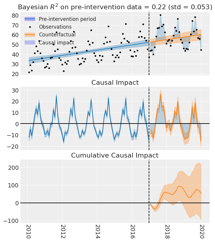
During the Post-period (2017-01-31 00:00:00 to 2019-12-31 00:00:00), the response variable had an average value of approx. 57.73. By contrast, in the absence of an intervention, we would have expected an average response of 56.29. The 95% interval of this counterfactual prediction is [51.74, 60.76]. Subtracting this prediction from the observed response yields an estimate of the causal effect the intervention had on the response variable. This effect is 1.45 with a 95% interval of [-3.03, 6.00].

Summing up the individual data points during the Post-period, the response variable had an overall value of 2078.37. By contrast, had the intervention not taken place, we would have expected a sum of 2026.27. The 95% interval of this prediction is [1862.54, 2187.30]. The cumulative effect is 52.10 with a 95% HDI [-108.93, 215.83].

The posterior probability of an increase is 0.735. For the cumulative effect, The posterior probability of an increase is 0.735. Relative to the counterfactual, the effect represents a 2.74% change (95% HDI [-4.98%, 11.59%]).

This analysis assumes that the relationship between the time-based predictors and the response observed during the pre-intervention period remains stable throughout the post-intervention period. If the formula includes external covariates, it further assumes they were not themselves affected by the intervention. We recommend inspecting model fit, examining pre-intervention trends, and conducting sensitivity analyses (e.g., placebo tests) to support any causal conclusions drawn from this analysis.

Pipeline approach#

The pipeline wraps these steps into a single, declarative workflow. Each step is configured upfront, and the pipeline validates everything before running.

df = (
    cp.load_data("its")
    .assign(date=lambda x: pd.to_datetime(x["date"]))
    .set_index("date")
)

result = cp.Pipeline(
    data=df,
    steps=[
        cp.EstimateEffect(
            method=cp.InterruptedTimeSeries,
            treatment_time=pd.to_datetime("2017-01-01"),
            formula="y ~ 1 + t",
            model=cp.pymc_models.LinearRegression(sample_kwargs={"random_seed": 42}),
        ),
        cp.GenerateReport(include_plots=False),
    ],
).run()

print("Experiment type:", type(result.experiment).__name__)
print("Effect summary available:", result.effect_summary is not None)
print("Report generated:", result.report is not None)

Initializing NUTS using jitter+adapt_diag...

Multiprocess sampling (4 chains in 4 jobs)

NUTS: [beta, y_hat_sigma]

Sampling 4 chains for 1_000 tune and 1_000 draw iterations (4_000 + 4_000 draws total) took 1 seconds.

Sampling: [y_hat]

Sampling: [y_hat]

Sampling: [y_hat]

Sampling: [y_hat]

Sampling: [beta, y_hat, y_hat_sigma]

Sampling: [y_hat]

Sampling: [y_hat]

Experiment type: InterruptedTimeSeries
Effect summary available: True
Report generated: True

Adding sensitivity analysis#

The SensitivityAnalysis step runs a suite of diagnostic checks against the fitted experiment. Checks are pluggable, and you can choose which ones to run.

result = cp.Pipeline(
    data=df,
    steps=[
        cp.EstimateEffect(
            method=cp.InterruptedTimeSeries,
            treatment_time=pd.to_datetime("2017-01-01"),
            formula="y ~ 1 + t",
            model=cp.pymc_models.LinearRegression(sample_kwargs={"random_seed": 42}),
        ),
        cp.SensitivityAnalysis(
            checks=[
                cp.checks.PlaceboInTime(n_folds=2),
            ]
        ),
        cp.GenerateReport(include_plots=True),
    ],
).run()

print(f"Sensitivity checks run: {len(result.sensitivity_results)}")
for check_result in result.sensitivity_results:
    print(f"  - {check_result.check_name}: {check_result.text[:80]}...")

Initializing NUTS using jitter+adapt_diag...

Multiprocess sampling (4 chains in 4 jobs)

NUTS: [beta, y_hat_sigma]

Sampling 4 chains for 1_000 tune and 1_000 draw iterations (4_000 + 4_000 draws total) took 1 seconds.

Sampling: [y_hat]

Sampling: [y_hat]

Sampling: [y_hat]

Sampling: [y_hat]

Sampling: [beta, y_hat, y_hat_sigma]

Sampling: [y_hat]

Sampling: [y_hat]

Initializing NUTS using jitter+adapt_diag...

Multiprocess sampling (4 chains in 4 jobs)

NUTS: [beta, y_hat_sigma]

Sampling 4 chains for 1_000 tune and 1_000 draw iterations (4_000 + 4_000 draws total) took 1 seconds.

Sampling: [y_hat]

Sampling: [y_hat]

Sampling: [y_hat]

Sampling: [y_hat]

Sampling: [beta, y_hat, y_hat_sigma]

Sampling: [y_hat]

Sampling: [y_hat]

/Users/benjamv/git/CausalPy/causalpy/steps/sensitivity.py:209: UserWarning: PlaceboInTime skipped folds because 1 fold(s) had pre-treatment history shorter than one full intervention window. Use fewer folds or an experiment_factory tailored to the eligible fold data; skipped_folds metadata records the observed and required pre-period rows.

../_images/65a4b36f5c3e4a8c907ca424e3dfc6863e6e39d22bb3f9cd4a6a39eef4793bce.png

Sensitivity checks run: 1
  - PlaceboInTime: Placebo-in-time analysis: 1 of 2 folds completed (1 skipped).
INCONCLUSIVE — onl...

Available checks#

CausalPy provides a range of sensitivity checks, each applicable to specific experiment types:

Check	Applicable methods	Description
`PlaceboInTime`	ITS, SC	Shifts treatment time backward to test for spurious effects
`PriorSensitivity`	All Bayesian	Re-fits with different priors
`ConvexHullCheck`	SC	Validates treated values are within control range
`PersistenceCheck`	ITS (3-period)	Checks if effects persist after intervention ends
`PreTreatmentPlaceboCheck`	Staggered DiD	Validates parallel trends via pre-treatment effects
`BandwidthSensitivity`	RD, RKink	Re-fits with multiple bandwidths
`LeaveOneOut`	SC	Drops each control unit and refits
`PlaceboInSpace`	SC	Treats each control as placebo treated
`McCraryDensityTest`	RD	Tests for running variable manipulation

Pipeline result#

The PipelineResult object contains all accumulated outputs:

print("result.experiment      ->", type(result.experiment).__name__)
print("result.effect_summary  ->", type(result.effect_summary).__name__)
print("result.sensitivity_results ->", len(result.sensitivity_results), "checks")
print("result.report          ->", "HTML" if result.report else "None")

result.experiment      -> InterruptedTimeSeries
result.effect_summary  -> EffectSummary
result.sensitivity_results -> 1 checks
result.report          -> HTML

The effect summary provides both a table and prose:

if result.effect_summary is not None:
    print(result.effect_summary.text)
    display(result.effect_summary.table)

During the Post-period (2017-01-31 00:00:00 to 2019-12-31 00:00:00), the response variable had an average value of approx. 57.73. By contrast, in the absence of an intervention, we would have expected an average response of 56.29. The 95% interval of this counterfactual prediction is [51.74, 60.76]. Subtracting this prediction from the observed response yields an estimate of the causal effect the intervention had on the response variable. This effect is 1.45 with a 95% interval of [-3.03, 6.00].

Summing up the individual data points during the Post-period, the response variable had an overall value of 2078.37. By contrast, had the intervention not taken place, we would have expected a sum of 2026.27. The 95% interval of this prediction is [1862.54, 2187.30]. The cumulative effect is 52.10 with a 95% HDI [-108.93, 215.83].

The posterior probability of an increase is 0.735. For the cumulative effect, The posterior probability of an increase is 0.735. Relative to the counterfactual, the effect represents a 2.74% change (95% HDI [-4.98%, 11.59%]).

This analysis assumes that the relationship between the time-based predictors and the response observed during the pre-intervention period remains stable throughout the post-intervention period. If the formula includes external covariates, it further assumes they were not themselves affected by the intervention. We recommend inspecting model fit, examining pre-intervention trends, and conducting sensitivity analyses (e.g., placebo tests) to support any causal conclusions drawn from this analysis.

	mean	median	hdi_lower	hdi_upper	p_gt_0	relative_mean	relative_hdi_lower	relative_hdi_upper
average	1.447234	1.485035	-3.025813	5.995170	0.7345	2.742124	-4.980082	11.587711
cumulative	52.100437	53.461271	-108.929252	215.826109	0.7345	2.742124	-4.980082	11.587711

Viewing the HTML report#

The GenerateReport step renders the full analysis — effect summary, diagnostic plots, and sensitivity-check results — into a single HTML report stored in result.report. See the report generation notebook for the standalone (non-pipeline) API.