Excess deaths due to COVID-19

import pandas as pd
from pymc_extras.prior import Prior

import causalpy as cp

%load_ext autoreload
%autoreload 2
%config InlineBackend.figure_format = 'retina'
seed = 42

Load data

df = (
    cp.load_data("covid")
    .assign(date=lambda x: pd.to_datetime(x["date"]))
    .set_index("date")
)

treatment_time = pd.to_datetime("2020-01-01")
df.head()

	temp	deaths	year	month	t	pre
date
2006-01-01	3.8	49124	2006	1	0	True
2006-02-01	3.4	42664	2006	2	1	True
2006-03-01	3.9	49207	2006	3	2	True
2006-04-01	7.4	40645	2006	4	3	True
2006-05-01	10.7	42425	2006	5	4	True

The columns are:

• date + year: self explanatory

• month: month, numerically encoded. Needs to be treated as a categorical variable

• temp: average UK temperature (Celsius)

• t: time

• pre: boolean flag indicating pre or post intervention

Run the analysis

In this example we are going to standardize the data. So we have to be careful in how we interpret the inferred regression coefficients, and the posterior predictions will be in this standardized space.

Note

The random_seed keyword argument for the PyMC sampler is not necessary. We use it here so that the results are reproducible.

model = cp.pymc_models.LinearRegression(
    sample_kwargs={"random_seed": seed},
    priors={
        "beta": Prior(
            "Normal",
            mu=[42_000, 0, 0, 0, 0, 0, 0, 0, 0, 0, 0, 0, 0, 0],
            sigma=10_000,
            dims=["treated_units", "coeffs"],
        ),
        "y_hat": Prior(
            "Normal",
            sigma=Prior("HalfNormal", sigma=10_000, dims=["treated_units"]),
            dims=["obs_ind", "treated_units"],
        ),
    },
)

result = cp.InterruptedTimeSeries(
    df,
    treatment_time,
    formula="standardize(deaths) ~ 0 + standardize(t) + C(month) + standardize(temp)",
    model=model,
).fit()

Initializing NUTS using jitter+adapt_diag...

Multiprocess sampling (4 chains in 4 jobs)

NUTS: [beta, y_hat_sigma]

Sampling 4 chains for 1_000 tune and 1_000 draw iterations (4_000 + 4_000 draws total) took 3 seconds.

Sampling: [y_hat]

Sampling: [y_hat]

Sampling: [y_hat]

Sampling: [y_hat]

Sampling: [beta, y_hat, y_hat_sigma]

Sampling: [y_hat]

Sampling: [y_hat]

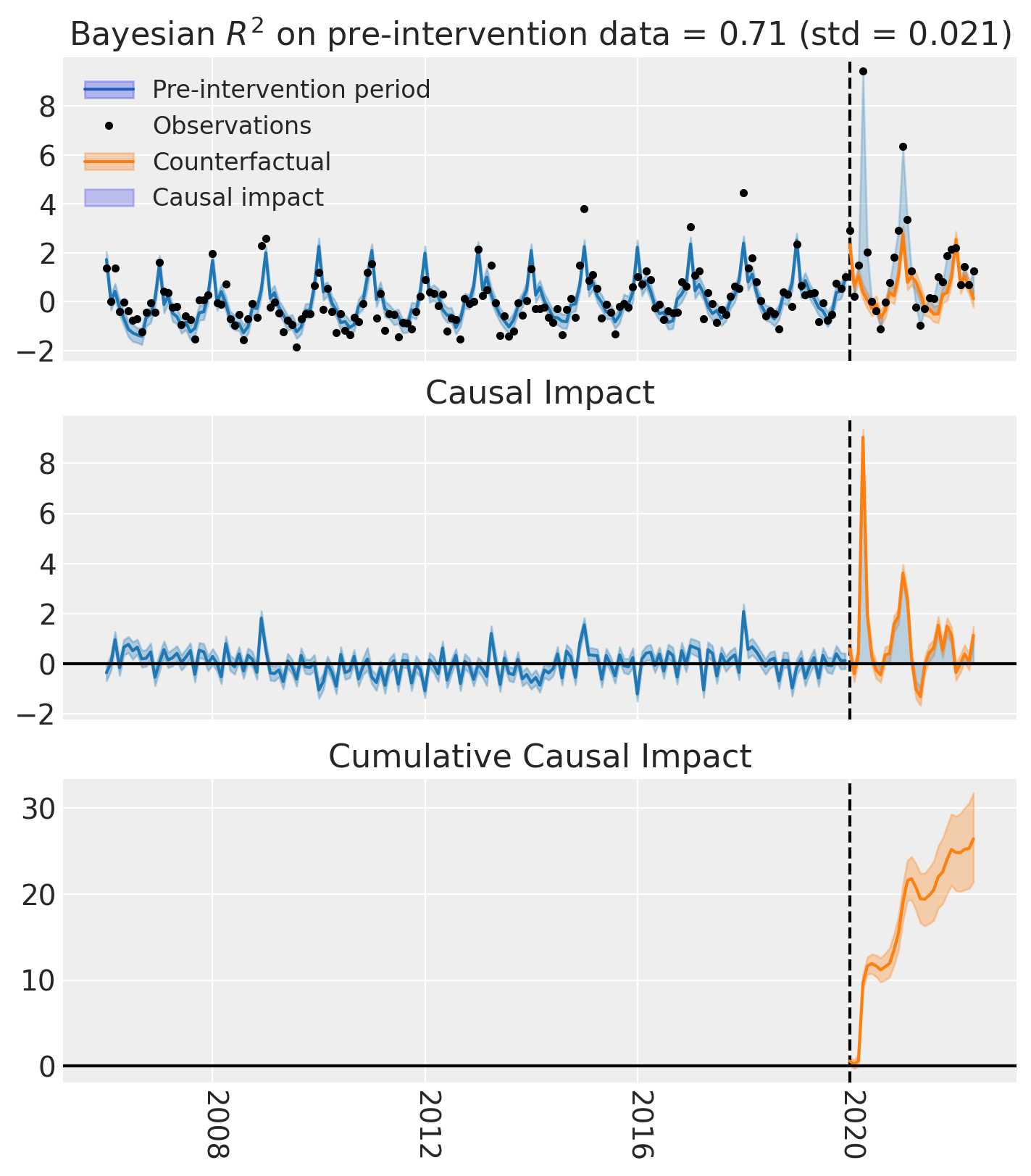
fig, ax = result.plot()

result.summary()

==================================Pre-Post Fit==================================
Formula: standardize(deaths) ~ 0 + standardize(t) + C(month) + standardize(temp)
Model coefficients:
  C(month)[1]        1.6, 94% HDI [1.1, 2]
  C(month)[2]        -0.22, 94% HDI [-0.67, 0.25]
  C(month)[3]        0.25, 94% HDI [-0.14, 0.63]
  C(month)[4]        -0.04, 94% HDI [-0.32, 0.25]
  C(month)[5]        -0.15, 94% HDI [-0.46, 0.15]
  C(month)[6]        -0.2, 94% HDI [-0.6, 0.24]
  C(month)[7]        -0.0031, 94% HDI [-0.53, 0.52]
  C(month)[8]        -0.4, 94% HDI [-0.89, 0.086]
  C(month)[9]        -0.43, 94% HDI [-0.83, -0.034]
  C(month)[10]       -0.055, 94% HDI [-0.35, 0.23]
  C(month)[11]       -0.37, 94% HDI [-0.73, -0.052]
  C(month)[12]       0.059, 94% HDI [-0.37, 0.52]
  standardize(t)     0.23, 94% HDI [0.16, 0.31]
  standardize(temp)  -0.46, 94% HDI [-0.77, -0.17]

Effect Summary Reporting

For decision-making, you often need a concise summary of the causal effect with key statistics. The effect_summary() method provides a decision-ready report with average and cumulative effects, HDI intervals, tail probabilities, and relative effects. This provides a comprehensive summary without manual post-processing.

Note

Note that in this example, the data has been standardized, so the effect estimates are in standardized units. When interpreting the results, keep in mind that the effects are relative to the standardized scale of the outcome variable.

# Generate effect summary for the full post-period
stats = result.effect_summary()
stats.table

	mean	median	hdi_lower	hdi_upper	p_gt_0	relative_mean	relative_hdi_lower	relative_hdi_upper
average	0.911757	0.912686	0.726295	1.097464	1.0	180.678877	92.777603	296.320675
cumulative	26.440939	26.467903	21.062542	31.826455	1.0	180.678881	92.777605	296.320683

# View the prose summary
print(stats.text)

During the Post-period (2020-01-01 00:00:00 to 2022-05-01 00:00:00), the response variable had an average value of approx. 1.45. By contrast, in the absence of an intervention, we would have expected an average response of 0.53. The 95% interval of this counterfactual prediction is [0.35, 0.72]. Subtracting this prediction from the observed response yields an estimate of the causal effect the intervention had on the response variable. This effect is 0.91 with a 95% interval of [0.73, 1.10].

Summing up the individual data points during the Post-period, the response variable had an overall value of 41.93. By contrast, had the intervention not taken place, we would have expected a sum of 15.49. The 95% interval of this prediction is [10.11, 20.87]. The cumulative effect is 26.44 with a 95% HDI [21.06, 31.83].

The posterior probability of an increase is 1.000. For the cumulative effect, The posterior probability of an increase is 1.000. Relative to the counterfactual, the effect represents a 180.68% change (95% HDI [92.78%, 296.32%]).

This analysis assumes that the relationship between the time-based predictors and the response observed during the pre-intervention period remains stable throughout the post-intervention period. If the formula includes external covariates, it further assumes they were not themselves affected by the intervention. We recommend inspecting model fit, examining pre-intervention trends, and conducting sensitivity analyses (e.g., placebo tests) to support any causal conclusions drawn from this analysis.

# You can also analyze a specific time window, e.g., the first 6 months of 2020
stats_window = result.effect_summary(
    window=(pd.to_datetime("2020-01-01"), pd.to_datetime("2020-06-30"))
)
stats_window.table

	mean	median	hdi_lower	hdi_upper	p_gt_0	relative_mean	relative_hdi_lower	relative_hdi_upper
average	1.986201	1.987324	1.802700	2.195508	1.0	293.672075	192.639518	419.492733
cumulative	11.917205	11.923943	10.816199	13.173046	1.0	293.672079	192.639520	419.492740

We can get nicely formatted tables from our integration with the maketables package.

from maketables import ETable

ETable(result, coef_fmt="b:.3f")

	standardize(deaths)
	(1)
coef
month=1	1.553
month=2	-0.216
month=3	0.253
month=4	-0.040
month=5	-0.147
month=6	-0.200
month=7	-0.003
month=8	-0.399
month=9	-0.430
month=10	-0.055
month=11	-0.373
month=12	0.059
standardize(t)	0.233
standardize(temp)	-0.458
stats
N	197
Bayesian R2	0.711
Format of coefficient cell: Coefficient